Breast Cancer

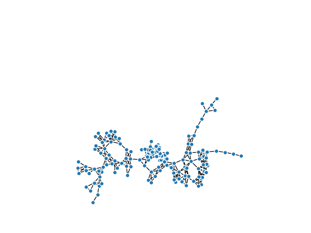
This example generates a Mapper built from the Wisconsin Breast Cancer Dataset.

The reasoning behind the choice of lenses in the demonstration below is:

• For lens1: Lenses that make biological sense; in other words, lenses that highlight special features in the data, that I know about.

• For lens2: Lenses that disperse the data, as opposed to clustering many points together.

In the case of this particular data, using an anomaly score (in this case calculated using the IsolationForest from sklearn) makes biological sense since cancer cells are anomalous. For the second lens, we use the \(l^2\) norm.

For an interactive exploration of lens for the breast cancer, see the Choosing a lens notebook.

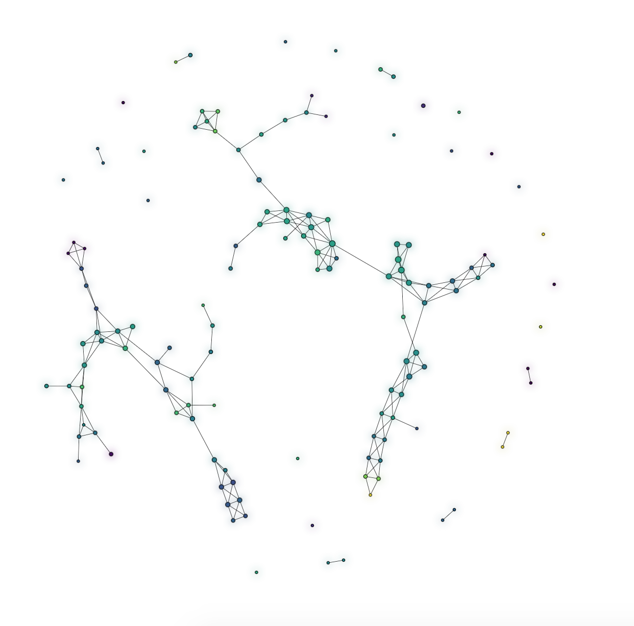
KeplerMapper also permits setting multiple datapoint color functions and node color functions in its html visualizations. The example code below demonstrates three ways this might be done. The rendered visualizations are also viewable:

• Visualization of the breat cancer mapper using multiple datapoint color functions

• Visualization of the breat cancer mapper using multiple node color functions

• Visualization of the breat cancer mapper using multiple datapoint and node color functions

Out:

KeplerMapper(verbose=3)
..Composing projection pipeline of length 1:
        Projections: l2norm
        Distance matrices: False
        Scalers: MinMaxScaler()
..Projecting on data shaped (569, 31)

..Projecting data using: l2norm

..Scaling with: MinMaxScaler()

Mapping on data shaped (569, 31) using lens shaped (569, 2)

Minimal points in hypercube before clustering: 2
Creating 225 hypercubes.
Cube_0 is empty.

Cube_1 is empty.

Cube_2 is empty.

Cube_3 is empty.

Cube_4 is empty.

Cube_5 is empty.

Cube_6 is empty.

Cube_7 is empty.

Cube_8 is empty.

Cube_9 is empty.

Cube_10 is empty.

Cube_11 is empty.

Cube_12 is empty.

Cube_13 is empty.

   > Found 2 clusters in hypercube 14.
Cube_15 is empty.

Cube_16 is empty.

Cube_17 is empty.

Cube_18 is empty.

   > Found 2 clusters in hypercube 19.
Cube_20 is empty.

   > Found 2 clusters in hypercube 21.
Cube_22 is empty.

Cube_23 is empty.

Cube_24 is empty.

   > Found 2 clusters in hypercube 25.
   > Found 2 clusters in hypercube 26.
   > Found 2 clusters in hypercube 27.
   > Found 2 clusters in hypercube 28.
Cube_29 is empty.

Cube_30 is empty.

Cube_31 is empty.

   > Found 2 clusters in hypercube 32.
Cube_33 is empty.

   > Found 2 clusters in hypercube 34.
Cube_35 is empty.

Cube_36 is empty.

   > Found 2 clusters in hypercube 37.
   > Found 2 clusters in hypercube 38.
   > Found 2 clusters in hypercube 39.
   > Found 2 clusters in hypercube 40.
Cube_41 is empty.

   > Found 2 clusters in hypercube 42.
   > Found 2 clusters in hypercube 43.
   > Found 2 clusters in hypercube 44.
Cube_45 is empty.

Cube_46 is empty.

   > Found 2 clusters in hypercube 47.
Cube_48 is empty.

   > Found 2 clusters in hypercube 49.
   > Found 2 clusters in hypercube 50.
   > Found 2 clusters in hypercube 51.
   > Found 2 clusters in hypercube 52.
   > Found 2 clusters in hypercube 53.
   > Found 2 clusters in hypercube 54.
   > Found 2 clusters in hypercube 55.
   > Found 2 clusters in hypercube 56.
   > Found 2 clusters in hypercube 57.
   > Found 2 clusters in hypercube 58.
   > Found 2 clusters in hypercube 59.
   > Found 2 clusters in hypercube 60.
   > Found 2 clusters in hypercube 61.
   > Found 2 clusters in hypercube 62.
   > Found 2 clusters in hypercube 63.
   > Found 2 clusters in hypercube 64.
   > Found 2 clusters in hypercube 65.
   > Found 2 clusters in hypercube 66.
   > Found 2 clusters in hypercube 67.
   > Found 2 clusters in hypercube 68.
   > Found 2 clusters in hypercube 69.
   > Found 2 clusters in hypercube 70.
Cube_71 is empty.

   > Found 2 clusters in hypercube 72.
   > Found 2 clusters in hypercube 73.
   > Found 2 clusters in hypercube 74.
   > Found 2 clusters in hypercube 75.
   > Found 2 clusters in hypercube 76.
   > Found 2 clusters in hypercube 77.
   > Found 2 clusters in hypercube 78.
   > Found 2 clusters in hypercube 79.
   > Found 2 clusters in hypercube 80.
   > Found 2 clusters in hypercube 81.
   > Found 2 clusters in hypercube 82.
   > Found 2 clusters in hypercube 83.
   > Found 2 clusters in hypercube 84.
   > Found 2 clusters in hypercube 85.
   > Found 2 clusters in hypercube 86.
   > Found 2 clusters in hypercube 87.
   > Found 2 clusters in hypercube 88.
   > Found 2 clusters in hypercube 89.
   > Found 2 clusters in hypercube 90.
   > Found 2 clusters in hypercube 91.
   > Found 2 clusters in hypercube 92.
   > Found 2 clusters in hypercube 93.
   > Found 2 clusters in hypercube 94.
   > Found 2 clusters in hypercube 95.
Cube_96 is empty.

   > Found 2 clusters in hypercube 97.
   > Found 2 clusters in hypercube 98.
   > Found 2 clusters in hypercube 99.
   > Found 2 clusters in hypercube 100.
   > Found 2 clusters in hypercube 101.
   > Found 2 clusters in hypercube 102.
   > Found 2 clusters in hypercube 103.
   > Found 2 clusters in hypercube 104.
   > Found 2 clusters in hypercube 105.
   > Found 2 clusters in hypercube 106.
   > Found 2 clusters in hypercube 107.
   > Found 2 clusters in hypercube 108.
Cube_109 is empty.

   > Found 2 clusters in hypercube 110.
   > Found 2 clusters in hypercube 111.
   > Found 2 clusters in hypercube 112.
   > Found 2 clusters in hypercube 113.

Created 304 edges and 158 nodes in 0:00:00.672039.
Wrote visualization to: output/breast-cancer.html
Wrote visualization to: output/breast-cancer-multiple-color-functions.html
Wrote visualization to: output/breast-cancer-multiple-node-color-functions.html
Wrote visualization to: output/breast-cancer-multiple-color-functions-and-multiple-node-color-functions.html
no display found. Using non-interactive Agg backend

import sys

try:
    import pandas as pd
except ImportError as e:
    print(
        "pandas is required for this example. Please install with `pip install pandas` and then try again."
    )
    sys.exit()

import numpy as np
import kmapper as km
import sklearn
from sklearn import ensemble

# For data we use the Wisconsin Breast Cancer Dataset
# Via:
df = pd.read_csv("data/breast-cancer.csv")
feature_names = [c for c in df.columns if c not in ["id", "diagnosis"]]
df["diagnosis"] = df["diagnosis"].apply(lambda x: 1 if x == "M" else 0)
X = np.array(df[feature_names].fillna(0))  # quick and dirty imputation
y = np.array(df["diagnosis"])

# We create a custom 1-D lens with Isolation Forest
model = ensemble.IsolationForest(random_state=1729)
model.fit(X)
lens1 = model.decision_function(X).reshape((X.shape[0], 1))

# We create another 1-D lens with L2-norm
mapper = km.KeplerMapper(verbose=3)
lens2 = mapper.fit_transform(X, projection="l2norm")

# Combine both lenses to create a 2-D [Isolation Forest, L^2-Norm] lens
lens = np.c_[lens1, lens2]

# Create the simplicial complex
graph = mapper.map(
    lens,
    X,
    cover=km.Cover(n_cubes=15, perc_overlap=0.4),
    clusterer=sklearn.cluster.KMeans(n_clusters=2, random_state=1618033),
)

# Visualization
mapper.visualize(
    graph,
    path_html="output/breast-cancer.html",
    title="Wisconsin Breast Cancer Dataset",
    custom_tooltips=y,
)


# Visualization with multiple color functions
mapper.visualize(
    graph,
    path_html="output/breast-cancer-multiple-color-functions.html",
    title="Wisconsin Breast Cancer Dataset",
    custom_tooltips=y,
    color_values=lens,
    color_function_name=["Isolation Forest", "L2-norm"],
)


# Visualization with multiple node color functions
mapper.visualize(
    graph,
    path_html="output/breast-cancer-multiple-node-color-functions.html",
    title="Wisconsin Breast Cancer Dataset",
    custom_tooltips=y,
    node_color_function=["mean", "std", "median", "max"],
)

# Visualization showing both multiple color functions, and also multiple node color functions
mapper.visualize(
    graph,
    path_html="output/breast-cancer-multiple-color-functions-and-multiple-node-color-functions.html",
    title="Wisconsin Breast Cancer Dataset",
    custom_tooltips=y,
    color_values=lens,
    color_function_name=["Isolation Forest", "L2-norm"],
    node_color_function=["mean", "std", "median", "max"],
)


import matplotlib.pyplot as plt

km.draw_matplotlib(graph)
plt.show()